What Type of Statistical Test to Use on Pre/post Test After Intervention

The evaluation of change is a primal goal in all sciences. In psychological, didactics, and medical sciences, there is a long tradition of using outcome size measures both to quantify the corporeality of change experienced past a group beyond several time points, and for comparing such modify in multiple groups (Cohen, 1988; Richardson, 1996; Fritz et al., 2012; Grissom and Kim, 2012; Kelley and Preacher, 2012; Pek and Flora, 2018). This paper examines the cess of modify through individuals' responses to standardized tests. Specifically, we focus on situations in which the same variable is measured at two time points in all the individuals in the sample (i.east., Pre-post research designs).

Pre-post designs are often used when an intervention is practical between the two time points. Whether the observed change can exist attributed to the intervention or not depends on a number of factors, including whether (a) a control group exists; (b) the study is experimental, quasi-experimental or observational; (c) relevant covariates and cofounds have been adequately controlled (Fisher, 1935; Rubin, 1974; Shadish et al., 2002; Pearl, 2009; Mayer et al., 2016).

Very oft, researchers want to crusade a change with their interventions. Some examples are: (a) A school instructor applying a visual-spatial preparation program to children of ages 10–12 would want them to increment their ability (c.f. Lowrie et al., 2017); (b) Numerous programs for cerebral training are intended to increase working memory capacity—and, ultimately, full general cerebral power—in their participants (c.f. Jaeggi et al., 2008); (c) Interventions with teenagers with autism spectrum disorders typically aim at improving their interpersonal and communication skills, among others; (d) Interventions in clinical psychology typically are intended to change the clients' behavior so they can adapt better to their environs and increment their quality of life (due east.g., gain social skills, command their anger or anxiety, improve their depressive symptoms, or avoid their maladaptive behaviors, among others; c.f. Muroff et al., 2014); (east) A pharmacological treatment for obesity volition be successful if the patients reduce their weight (c.f. Pi-Sunyer et al., 2015)¹.

In a pre-mail enquiry blueprint, some criterion is needed to determine large or small change. Here we focus on distribution based methods (i.e., there is no external information or clinical referents, other than the exam scores; Lydick and Epstein, 1993; Crosby et al., 2003; Revicki et al., 2008). These methods attempt to place the smallest change that cannot be explained by sampling random fluctuations or by measurement fault (Jacobson and Truax, 1991; Crosby et al., 2003; Bauer et al., 2004). This amount of modify is unremarkably called statistically reliable, minimally detectable or just reliable alter (Maassen, 2000; Beaton et al., 2001; de Vet et al., 2006).

To detect a reliable change, two approaches can exist adopted. Nosotros termed them the average-based change approach (ABC) and the individual-based modify approach (IBC). The aim of ABC is to evaluate whether a grouping, as a whole, experienced a reliable alter. In turn, the goal of IBC is to place specific individuals who showed change. To appraise ABC, researchers often use a statistic that describes the middle of the distributions (oft, the pre and mail service means), by using zippo hypothesis tests and upshot size measures (c.f., Cohen, 1988; Fritz et al., 2012; Grissom and Kim, 2012; Pek and Flora, 2018). To assess IBC, researchers may use diverse indices that can be grouped nether the proper name of reliable change indices. Some of these indices are based on standardization of pre-post differences, others on the standard fault of measurement, and nonetheless others on linear regression predictions (Crosby et al., 2003; Ferrer and Pardo, 2014).

The goal of this newspaper is twofold. Starting time, we want to investigate the relation betwixt ABC and IBC statistics, and to describe such a relation in mathematical terms. Nosotros show that, contrary to what other previous studies have speculated, both approaches are strongly related. 2nd, we attempt to draw researchers' attending to a set of tools derived from private-based statistics. These are elementary tools that can provide help in a diverseness of research contexts. We bear witness how they can exist used for intuitive interpretation and communication of inquiry results, and how they can supercede capricious cutoffs (eastward.g., Cohen, 1988) unremarkably used for deciding when an effect is "small" or "large."

Are the Average-Based and the Private-Based Approaches Related?

Many studies have argued that the information provided by these two approaches is dissimilar. Beneath are some examples:

"Statistical methods based on the General(ized) Linear Model (…) have optimal power when individuals conduct identically (…). When there exists genuine, idiosyncratic variations in the effect of a factor, (…) the effect of a cistron can be significant for every individual (…) while Educatee and Fisher tests yield a probability close to 1 if the population average is small enough" (Vindras et al., 2012, p. 2).

"Statistically significant change at the group level may not be meaning at the individual level (…). Hateful changes for a group may be the result of few individuals with relatively large changes, or numerous individuals with relatively pocket-size changes" (Schmitt and Di Fabio, 2004, pp. 1008–1009).

Similar ideas can be found in other studies (due east.thou., Ottenbacher et al., 1988; Testa, 2000). Accordingly, it appears that average and individual approaches focus on different aspects of change, inasmuch as knowing that the center of the scores distribution changed provides no information about which item individuals inverse. Indeed, the modify in the distribution center and the percentage of individual changes are calculated in very different ways.²

However, it is not axiomatic whether these two approaches are completely contained. Rather, information technology is reasonable to recall that the larger the displacement of distribution heart, the higher the percentage of reliable individual changes. In fact, the higher the mean of the pre-post differences, the more than likely it is that a pre-mail deviation exceeds a sure cutoff. For example, if the pre-mail service differences distribution is normal, the probability associated with each cutoff is known. If the hateful of the differences equals zero, the probability of finding cases to a higher place 1.645 standard deviations equals 0.05. If the mean of the differences is 0.5 standard deviations above zero, the probability of finding cases in a higher place 1.645 standard deviations equals 0.thirteen, etc. However, these probabilities are unknown when the pre-post differences distribution is non-normal, which is the usual instance in applied contexts.

One study showed that the pre-post event size observed (i.e., the magnitude of change in distribution eye) is the principal determinant of the percentage of individuals showing pre-post change (Norman et al., 2001). This simulation report revealed that the relation betwixt effect size and percentage of change is approximately linear for upshot sizes beneath ane, with normal and moderately skewed distributions, and regardless of the cutoff to detect a change. Therefore, at least under certain conditions, the mean change can yield some information about the percentage of private changes. A later written report using empirical data constitute consequent results (Lemieux et al., 2007). However, these papers did not report any mathematical function to estimate the percentage of changes based on the change in the distribution center, nor did they report the fit that such a role may reach, which would be useful to assess the quality of its estimations.

The scarcity of studies on this topic and the lack of sound conclusions suggest that more inquiry is needed to understand the relation betwixt the change in the distribution center and the percent of individual changes.

The Present Study

Our first goal in this article was to investigate the relation betwixt ABC and IBC statistics, and to mathematically draw that relation. Specifically, nosotros sought to: (a) investigate whether ABC and IBC are related; (b) if and so, place its shape, a mathematical function that best represents it, and the goodness of fit of such function; and (c) determine what conditions touch on the nature of the relation. For this, we conducted a simulation study corresponding to ii of the most common designs in the behavioral and social sciences: a "pre-mail design" and a "control group pre-postal service design." To our cognition, this is the first study applying private alter indices to a pre-post design with a command grouping. Importantly, we studied this relation in scenarios with both normal and not-normal distributions.

Our second goal was to promote the use of individual-based statistics every bit a simple and useful tool for addressing important research questions. Based on our simulation results, we show that such statistics can exist used to translate research results and brand decisions in applied settings.

Methods

We simulated data for two scenarios in which the same variable is measured at ii time points (e.grand., before and after the intervention) for each individual inside a group of participants. We generated two different pre-post enquiry designs: with and without a control group.

Including a single grouping blueprint is important because: (a) this is a common scenario in practical contexts; and (b) all indices describing the per centum of private changes were adult for settings with a single treated group (Payne and Jones, 1957; Jacobson and Truax, 1991; Crawford et al., 1998; Hageman and Arrindell, 1999; Wyrwich et al., 1999). On the other mitt, it is well known that including a command group—ideally, with random assignment—provides stronger testify for attributing the change to the handling (Shadish et al., 2002; Feingold, 2009).

Simulation Conditions

To define the simulation conditions, nosotros manipulated four criteria (for a summary, run across Tabular array 1):

a. Effect size in the experimental/handling group (δ_exp = μ_dif.exp/σ_dif.exp). We computed the outcome size as the standardized hateful of the pre-postal service differences (Cohen, 1988; see the discussion and Appendix 1 in Supplementary Information Sheet 2 for considerations about using a dissimilar standardizer). We chose 13 consequence sizes ranging from 0 to 3.six with 0.3 betoken increases (e.one thousand., an effect size of 0.half dozen indicates that the mean of the pre-mail differences μ_dif.exp is 0.vi times the standard divergence of the individual pre-post differences σ_dif.exp). The rationale for choosing this broad range of effects, from a null result to an extremely large one, was to permit the percentage of individual changes to incorporate its full range (0–100%). In our analyses we assumed that the mean scores increased over time. To summate the differences, we subtracted pre-test score from the mail-examination score. Consequently, because we generated positive furnishings in our simulation, nosotros used right one-tailed tests.

In the single group pre-post design, we generated data for the treatment group just. In the command group pre-post pattern, we added data for a command group with no expected pre-post mean differences, (i.due east., δ_ctrl = 0). The values for the residuum of simulation criteria were the aforementioned for the command and treatment groups in every conditions (see beneath).

Importantly, this value was the mean effect size in the population. Centered on this hateful, a random distribution of individual changes was created, and each case within the sample experienced a different corporeality of alter. The variance of this distribution depended on the pre-postal service correlation (see betoken c below). Figure 1 depicts the pre, post and modify scores for 1 sample.

b. Sample size of each grouping (north). We chose three sample sizes (25, 50, and 100) to simulate what is usually considered small, medium, and large sample sizes in clinical work (Crawford and Howell, 1998). In the command group design, both groups had the same sample size.

c. Pre-mail service correlation (ρ_pre−post): 0.5, 0.vii, and 0.9. We chose these values to simulate a range of mutual correlations in applied settings (Pedhazur and Schmelkin, 1991; Nunnally and Bernstein, 1994. Note that correlations <0.5 are very uncommon in repeated measures settings). We used the Pearson's correlation coefficient. In the command grouping design, both groups were expected to have the same correlation value. With σ_pre = σ_post = i, these three values pb to a standard deviation of the differences (σ_dif) of 1, 0.775, and 0.447 respectively—i.eastward., higher pre-post correlation entails lower variance of the differences (See Appendix iii in Supplementary Information Sail 2 for a discussion on the consequence of measurement error).

d. Shape of the pre and post distributions. Given that moderate and severe deviations from normality are often constitute in applied contexts (Micceri, 1989; Blanca et al., 2013), we faux seven unlike conditions past modifying the degree of skewness (g ₁) and kurtosis (g _ii): (one) farthermost negative skewness: g _i = −3, g _ii = xviii; (2) moderate negative skewness: g ₁ = −2, k ₂ = 9; (3) mild negative skewness: g _one = −1, one thousand _two = ii; (4) normality: k ₁ = 0, g _ii = 0; (five) balmy positive skewness: g ₁ = ane, thousand _ii = two; (6) moderate positive skewness: k ₁ = 2, g ₂ = nine; and (7) farthermost positive skewness: g ₁ = iii, thousand ₂ = xviii. Note that the kurtosis is partially conditioned by the skewness. Less than 5% of existent data is expected to have more farthermost distributions (Blanca et al., 2013). In the control group design, both groups were expected to have the same shape for the pre- and post- distributions.

Table 1. Summary of simulation weather condition and computed statistics.

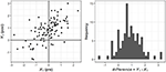
Figure ane. Pre, post and difference scores for ane sample of n = 100, with δ_exp = 1.2, ρ_pre−post = 0.seven, and normal distribution. Notation that the amount of alter is different for every individual.

Simulation Procedure

By combining the four criteria described in a higher place nosotros generated 13 × 3 × 3 × 7 = 819 dissimilar conditions for the simulation. For each of these weather, nosotros generated 500 samples (409,500 samples in total). This was washed separately for the simple pre-post blueprint (ane experimental group per sample) and for the control group pre-mail service design (one experimental and one command group per sample). We used MatLab 2011a to perform the simulation. The code is available in the Supplementary Data Sheet 1.

In the single grouping pattern, nosotros first generated a matrix X _i = (X _one*, Y _ane*) containing north pairs of scores in two non-correlated variables. Scores were generated by using Pearson's distribution system. Both variables had the aforementioned mean, standard departure, skewness, and kurtosis. The mean was always fixed to zero and the standard deviation was fixed to one. Skewness and kurtosis were systematically modified according to g _ane and yard ₂ values explained previously. Ten and Y were generated randomly to ensure that the post score may be the aforementioned, higher, much higher, lower or much lower than their corresponding pre-score, equally is typically the instance in existent information.

Second, nosotros fixed the correlation value between variables in 10 ₁ by applying the Cholesky covariance decomposition of correlation matrix R corresponding to the called correlation value (ρ_{pre−mail service}). The resulting matrix M _ane = (X ₁, Y ₁) contained two variables (X ₁ = pre; Y _i = mail) with skewness, kurtosis and ρ _XY (or ρ_pre−post) values similar to the specified ones. This transformation ensured that the post-scores were non independent of the pre-scores, equally is also the instance in real information. Note that, although simulating the divergence scores would be simpler and faster than simulating pre and post scores, information technology would make it incommunicable to study the effect of the pre-mail service correlation.

In the final step we modified Y ₁ to adjust it to the desired mean value in each status. For this purpose, we added the standard departure of pre-post differences, multiplied past the corresponding value of δ_exp, to each individual Y _i value.

In the control group design, the process was identical except for two changes: (a) instead of only one matrix in each replication, we generated a pair of independent matrices Ten ₁ = (X ₁*, Y ₁*) and Ten ₂ = (X _two*, Y ₂*) for simulating the scores of the experimental (X ₁ ) and control (Ten ₂ ) groups; and (b) we modified Y _i in the experimental matrix only to adapt information technology to the desired hateful value in each status (whereas the mean for Y ₂ was not inverse for the command group).

Importantly, this procedure ensured that every example experienced a different amount of change. Figure 1 depicts pre-, post- and difference scores for i sample of northward = 100, with δ_exp = ane.2, ρ_{pre−mail service} = 0.vii, and normal distribution.

Data Analysis

In the single grouping pre-post blueprint, we computed the empirical group or average change for each sample by computing the difference between the post- and the pre-test ways, and dividing such difference by the standard divergence of the differences,

$\begin{array}{rc}\mathit{\text{d}}=({\mathit{\text{M}}}_{\text{post}}-{\mathit{\text{M}}}_{\text{pre}})/{\mathit{\text{Due south}}}_{\text{dif}}& (1)\end{array}$

In this paper nosotros employ d to refer to the event of applying Equation 1. Run across the word and Appendix 1 in Supplementary Data Sheet 2 for a word on a dissimilar computation of the standardized hateful difference.

In the control grouping pre-post pattern, we quantified the average change by using the ω² statistic associated with the interaction betwixt the between-subjects gene A (group) and the inside-subjects cistron B (pre- and post-test). The internet change is captured past comparing the pre-post change in the experimental group with the pre-post modify in the control group (Hays, 1988; Kirk, 2013). For our design, ω^two tin can be estimated as

$\begin{array}{l}{\omega }^2=\frac{g{l}_{AB}(F_{AB}-1)}{g{l}_{AB}(F_{AB}-1)+\mathrm{North}},\end{array}$

were F _AB is the interaction F statistic, gl _AB are the interaction degrees of liberty, and N is the full number of scores in the design (adding both groups).

To identify which individual scores showed a reliable change (i.e., which cases roughshod in a higher place a certain cutoff after existence standardized) and then calculate the percentage of individual changes for each sample, we decided to utilize 2 individual alter indices. We chose two indices that take shown everyman false negative rates (come across Ferrer and Pardo, 2014).

a. Standardized individual difference (SID; Payne and Jones, 1957). The standardized score resulting from dividing the private pre-post difference (D _i ) by the standard departure of these differences (South _dif), as

This standardization was proposed to assess the degree of discrepancy between two scores (Payne and Jones, 1957). If the distribution of pre-mail divergence is normal, 95% of SID will fall betwixt ± ane.96 values, and ninety% between ± 1.645 values.

b. Reliable Change Index (RCI; Jacobson et al., 1984, 1999; Jacobson and Truax, 1991). This is probably the well-nigh popular private change alphabetize. It is based on the standard error of measurement. Of the several bachelor versions, we used one in which the equality of pre- and mail service-test variances is not assumed (see Christensen and Mendoza, 1986; Jacobson and Truax, 1991; Maassen, 2004). This version is specified as:

$\begin{array}{l}RCI=\frac{D_i}{\sqrt{{\left(S_{\mathrm{\text{pre}}}\sqrt{\mathrm{ane}-R_{\mathrm{\text{pre-postal service}}}}\right)}^2+{\left(S_{\mathrm{\text{mail}}}\sqrt{\mathrm{one}-R_{\mathrm{\text{pre-postal service}}}}\right)}^2}}.\end{array}$

Using this index, the lower simulated positive rate is achieved when reliability is estimated from the pre-postal service correlation (R _pre−post) (Ferrer and Pardo, 2014).

These two indices were computed for each individual case in all the fake samples. We considered an individual change to be reliable when its corresponding SID or RCI was higher than 1.96 (two-tailed test) or 1.645 (one-tailed test) points. In the single grouping pre-post design, nosotros applied one cutoff of 1.645. In the command group pre-post design we performed two-tailed tests (cutoffs of −1.96 and i.96) for all conditions because the procedure is intended to compare the effectiveness of 2 different treatments in real scenarios. Hence, information technology is important to take into consideration the proportion of worsened cases, non only the improved ones.

In the single group design, nosotros computed the percentage of reliable improvements for each sample. In the control grouping pattern, we computed the proportion of both worsened (P ⁻) and improved (P ⁺) cases in each group within the samples, and and then subtracted the issue for the command group (ctrl) from this same consequence in the experimental group (exp). This process yielded a cyberspace percent of positive changes attributable to treatment³(P _internet):

$\begin{array}{rc}{P}_{\mathrm{\text{cyberspace}}}=(P_{exp}^{+}-P_{exp}^{-})-(P_{\mathrm{\text{ctr}}}^{+}-P_{\mathrm{\text{ctr}}}^{-})& (2)\end{array}$

So we examined the relation betwixt the change estimated with ABC statistics and the alter estimated using IBC statistics by fitting several regression functions.

Finally, with each empirical effect size and percentage of private changes (500 pairs of values for each condition in the simulation, i.e., a pair by sample), we obtained: (a) a scatterplot to audit the underlying relation between the two statistics, and (b) several different regression functions to quantify the extent to which the change in the distribution center is predictive of the percentage of individual changes. This was done separately for each inquiry design.

Results

For brevity of presentation, we written report here the nigh representative results. For all conditions in both designs, the properties of the generated samples corresponded to those imposed in the simulation. We report the results regarding SID only; those based on the RCI are similar. Results from all atmospheric condition and based on the RCI are available upon request.

Unmarried Group Pre-Mail Design

To examine the relation between ABC and IBC, we first plotted the effect size measured by d (boilerplate-based alter) against the pct of individual changes (individual-based change). Figure two (top row) shows scatterplots based on SID alphabetize, for n = 100 and ρ_pre−post = 0.vii. Each of the points in these scatterplot depicts i of the simulated samples (i.eastward., 13 consequence sizes × 500 simulated samples = 6,500 points per scatterplot). The patterns with ρ_pre−post = 0.5 and ρ_{pre−postal service} = 0.9 were similar. We study here the weather with the largest sample size to illustrate the shape of the relation with greater clarity. The aforementioned blueprint is observed for due north = 25 and due north = 50, but with college variability. In other words, any particular d value corresponds to the same mean percent of changes, only a smaller sample size leads to more scattered points due to college sampling error.

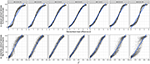
Effigy 2. Relation between average-based modify (horizontal centrality) and individual-based change (vertical centrality). Top row (A) shows the data for the simple grouping pre-mail design. Bottom row (B) shows the data for the pre-post pattern with a control group. Data based on SID with n = 100 and ρ_pre−post = 0.seven. Sk, skewness; Kr, Kurtosis.

To quantify the relations detected in Figure 2, we estimated four different regression functions: linear, quadratic, cubic, and logistic. In every case, d (average-based effect size) was used as the contained variable and the percentage of changes (individual-based outcome size) as the dependent variable.

Table two reports the coefficient of determination (R ²) for the four functions, for northward = 25. Because the dispersion in the various scatterplots decreases equally sample size increases, these R ² values were the lowest of all values. Nevertheless, fifty-fifty with north = 25, iii of the four functions provided an first-class fit. Beginning, the linear function achieves R ² values around 0.ninety in negatively skewed distributions and above 0.90 values in the remaining distributions, reaching 0.96. With due north = 50 and n = 100, R ² ranges between 0.91 and 0.98; the lowest values are observed in the conditions with more extreme skewness. Second, the quadratic function achieves R ² values similar to the linear role, although slightly higher in negative skewness conditions. Third, the cubic function yields R ² values betwixt 0.96 and 0.98, although at the price of introducing more complexity. Fourth, the logistic function yields the everyman values, between 0.68 and 0.78.

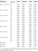
Table ii. R ² of linear, quadratic, cubic and logistic functions for the unmarried group design.

3 of the iv adjusted functions offered a very good fit to the information. Moreover, they offered very similar predictions. For example, with n = 25, ρ_pre−post = 0.70, and δ_exp = 1, the predicted value (the estimated percentage of changes) is 30.seven% for the linear function, 31.7% for the quadratic function, and 26.9% for the cubic function. Of these, the linear office is the most parsimonious, peculiarly for applied settings (Bentler and Mooijaart, 1989; Maxwell and Delaney, 2004; Steele and Douglas, 2006). Table iii reports the coefficients from the linear office. These coefficients can be used to gauge the percentage of private changes from the effect size d. Given that the value of the former tin can range from −100 to 100, the constant coefficient B ₀ is adequately close to zero in every instance (with absolute values ranging from 0.09 to ii.fifty, and standard errors <0.27; p > 0.05 in all cases), and the slope coefficient B _i is shut to 30 (28.75 to thirty.86, with standard fault < 0.12). Results with other atmospheric condition were similar in all regards.

Table 3. Coefficients (and standard errors) for the lineal regression model in the single grouping design.

Results from the linear function betoken that: (a) when issue size is cypher, the expected percent of changes (computed using SID) ranges betwixt 0 and iii%, and (b) for each actress point of outcome size, the expected percentage of changes rises by 30 points. Because prediction is done using percentages, values below nada and to a higher place 100 must be replaced by their respective limits.

Pre-Post Design With Command Group

Figure 2 (bottom row) shows the relation betwixt ${\widehat{\omega }}^2$ (boilerplate-based effect size measure) and the net percentage of changes (private-based effect size measure). The latter was calculated from SID (north = 100 and ρ_{pre−postal service} = 0.7). Each of the points in these scatterplot depicts one of the simulated samples comprising one command and ane experimental group. As in the meridian row, nosotros written report the results for the atmospheric condition with the largest sample size. The smaller sample sizes yielded the same blueprint yet with higher variability. Patterns with the other ρ_pre−post values were similar.

To quantify the relation observed in the bottom row of Effigy 2, we estimated four unlike regression functions: linear, quadratic, cubic and logistic. In every case, ${\widehat{\omega }}^2$ was used separately as the independent variable, and the internet percentage of individual changes served every bit the dependent variable. The 4 functions were estimated for each of the conditions faux. Table 4 reports the coefficient of determination (R ²) for these four functions. These results are based on net pct of private changes calculated with SID alphabetize and n = 25. Considering dispersion from the various scatterplots decreases as sample size increases, R ² values from Table 4 were lower than those achieved with n = 50 and n = 100.

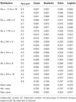
Table iv. R ^two of linear, quadratic, cubic and logistic functions for the n = 25 conditions of the control grouping pre-post blueprint.

Overall, the four functions achieved a very adept fit. The R ^two values were college when the distributions approached normality. The quadratic and cubic functions achieved a slightly better fit than the linear part, merely only with negative skewness; the logistic and linear functions achieved similar fit. As in the single grouping blueprint, the linear function was deemed preferable because it is the nigh parsimonious, with but minimal loss of fit.

In Table 5 (analogous to Tabular array 3 in the single group blueprint) we report the coefficients from the linear office with north = 25. These coefficients allow estimating the net percentage of individual changes from the upshot size measures. The intercept (B ₀) ranges from −0.04 to approximately 6, with a hateful of 2.41 and standard errors ranging between 0.xix and 0.33. The slope (B ₁) ranges from 140 to 165, with a mean of 153 and standard errors ranging between 0.53 and 0.91. As an case, if nosotros consider the results for the normal distributions, these coefficients indicate that for a null effect size (${\widehat{\omega }}^2$ = 0), the linear function yields an estimated net pct of changes of approximately 2.five%. For each boosted 0.10 points of ${\widehat{\omega }}^2$, the internet percent of changes increases in approximately xv points (as we are predicting percentages, values across goose egg, and 100 must be replaced by their corresponding limits). Note that the changes in pre-post correlation practise not essentially alter the coefficients B ₀ and B _one in Tabular array 5. Similar results were plant with the other sample sizes.

Tabular array 5. Coefficients (and standard errors) for the lineal regression model in the pattern with a command group.

Discussion

Our first goal in this newspaper was to make up one's mind whether ABC (quantified past d in the single group design or by ${\widehat{\omega }}^{\mathrm{two}}$ in the command group pattern) is related to IBC (quantified as the percent of private changes, or net pct in the control group design). Our simulations indicate that percentage of changes is related to average-based effect size. In all conditions, and for both designs, the results show that, as average-based effect size increases, so does the percentage of changes.

Inside this general goal, we aimed at finding a mathematical function to capture the relation between issue size and per centum of changes. In both designs, the adapted linear, quadratic and cubic functions showed splendid fit. The logistic function showed expert fit in the single grouping design, and first-class fit in the control group pattern. Amidst them, the linear model was the most parsimonious and easiest to interpret, and hence was preferred (Bentler and Mooijaart, 1989; Maxwell and Delaney, 2004; Steele and Douglas, 2006). Information technology showed excellent fit in all conditions fifty-fifty in the least favorable simulated scenarios (n = 25): the R ² values ranged from 0.90 to 0.96 in the single grouping blueprint (Table 2) and from 0.79 to 0.93 in the command group design (Tabular array 4).

Finally, nosotros wanted to identify conditions in which the ABC and IBC are related. Our results bespeak that such a relation was present in all faux weather and for both designs, regardless of the pre and mail distributions skewness, and of the pre-post correlation. The fit (R ^two) of the linear regression office slightly varied from 0.96, in the nearly favorable conditions, to 0.90 (unmarried grouping blueprint), and 0.79 (control group blueprint) in the nearly adverse. As sample size increases, so does fit: with n = 100, R ² reached 0.98 in the most favorable conditions, and was never below 0.87 in the most agin.

A very important finding from our report was that, for both designs, the slope of the regression line was approximately the same in all simulated conditions. In the single group design (with d as predictor and the pct of changes as dependent variable), the slope value was around thirty (ranging from 29 to 31). This indicates that, for each added point to the issue size, the office's estimation of the percentage of changes increased by 30 points. In other words, a 0.10-point increment in d (pre-post differences metric) was associated with a three-signal increase in the percentage of private changes⁴.

In the command group blueprint (with ${\widehat{\omega }}^2$ as predictor and the internet per centum of changes every bit the dependent variable), the slope value was around 153 points, ranging from 140 to 165. Because the values of ${\widehat{\omega }}^2$ range from 0 to 1, expressing it this way is more useful: for each 0.10 added points to the result size, the linear function estimate for the percentage of private changes increases in 15.3 points (ranging from xiv to 16.v).

Relevance of the Present Findings

Some important implications are worth noting: (a) The ABC and IBC statistics are near equivalent; and (b) Cutoffs commonly used for deciding when an effect is pocket-sized, medium or large should be replaced with more informative indices. Beneath, nosotros aggrandize on these ideas and offer 2 recommendations based on them.

The ABC and IBC Statistics Are Most Equivalent

With two exceptions (Norman et al., 2001; Lemieux et al., 2007), papers on this topic agree on the following idea: researchers will arrive to different conclusions about a treatment's effectiveness depending on whether they assess it at the individual or at the group level (e.g., Ottenbacher et al., 1988; Testa, 2000; Schmitt and Di Fabio, 2004; Vindras et al., 2012). Our results indicate that this idea is wrong. Across all of our simulation conditions, ABC and IBC statistics were so closely related that tin exist considered as dissimilar expressions of nearly the aforementioned information. This is to exist expected, indeed, when variability of pre- and mail-test scores is the same. Because increases in effect size lead to increases in the center of the pre-post differences distribution, the number of cases on the right side of whatever chosen cutoff volition likewise increase.

Based on this finding, we offer our first recommendation: When evaluating the change in a group, if only one pre- and 1 post- measures are bachelor, a logical sequence of analytic steps is every bit following: (a) assess individual changes through SID or RCI, (b) aggregate the individual results into a percentage of reliable private changes (or internet pct, if more than i group is analyzed), and, (c) study this individual-based statistics forth with classical average-based effect size estimations such as d or ${\widehat{\omega }}^{\mathrm{ii}}$.

This procedure has several advantages over merely reporting the ABC statistics. First, information technology allows researchers to make decisions about each particular case. This is a mutual business organization in applied settings, and the individual-based methods discussed here provide a straightforward tool for addressing information technology (Sijtsma, 2012). The usefulness and convenience of these indices have been discussed elsewhere (Jacobson and Truax, 1991; Maassen, 2000; Ferrer and Pardo, 2014). 2d, an effect size expressed as a percentage is easier to understand and it enhances the advice of results, especially among researchers without a strong statistical groundwork. For case, in a randomized controlled trial, stating that the effect size was ${\widehat{\omega }}^2$ = 0.20 is less articulate than stating that the observed internet pct of individual changes was 33%.

Recent recommendations advocate that effect size estimates should directly accost the research question which motivated their estimation, and should be intuitively accessible so that they facilitate the effective scrutiny of results (Pek and Flora, 2018). Nosotros fence that, when used for effect size estimation, individual-based statistics accomplish both aims. Based on this, and in line with previous work (due east.m., Ogles et al., 2001; Wise, 2004; Lambert and Ogles, 2009; Speelman and McGann, 2013; de Beurs et al., 2016; Fisher et al., 2018), nosotros encourage other researchers to include individual-based statistics in their methodological toolbox and to use them to report their results.

Another finding worth highlighting is that, because the intercept and slope coefficients were very similar across conditions, information technology is easy to compute an gauge pct (or net percentage) of reliable individual changes fifty-fifty without having access to the raw data. For example, if a researcher wants to express an already published effect size as a pct of changes, the but needed pace is to introduce the guess into the linear regression equation proposed in our results. For example, in a single group pre-post report with d = 0.ix with ordinarily distributed scores, and based on Table iii:

$\begin{array}{rc}Percenta\mathrm{yard}\mathrm{due\; east}ofcha\mathrm{northward}\mathrm{chiliad}\mathrm{east}s\approx B_0+B_1\times d=\mathrm{ane}.9+29\times 0.9\approx 28\%& (3)\end{array}$

In a command group pre-postal service study with ${\widehat{\omega }}^2$ = 0.4, with normally distributed scores, pre-postal service correlation of r = 0.7, and based on Tabular array 5:

$\begin{array}{rc}\mathrm{North}etp\mathrm{due\; east}rcentam\mathrm{eastward}ofcha\mathrm{northward}\mathrm{grand}e\mathrm{south}\approx {\mathit{\text{B}}}_0+{\mathit{\text{B}}}_{\mathrm{i}}\times {\widehat{\omega }}^{\mathrm{two}}=\mathrm{two}.6+152\times 0.\mathrm{four}\approx 63\%& (\mathrm{iv})\end{array}$

When d or ${\widehat{\omega }}^2$ are not bachelor in the published report, it is easy to compute them from other effect sizes estimates (encounter Appendix 1 in Supplementary Data Canvas two for examples of these computations, and see Appendix 2 in Supplementary Information Sheet 2 for an application to information from one published paper). The specific intercept and slope values can be selected co-ordinate to the empirical skewness and kurtosis (see Tables 3, 5). But even if coefficients from a wrong condition are selected, the estimate of the (net) percentage of changes will exist close to the real value.

Based on previous research (Blanca et al., 2013), less than 5% of existent datasets have more extreme distributions than the ones simulated here. Consequently, our simple linear regression models can be applied in most existent situations to estimate the approximate percentage of individuals who experienced change, when only average-based change indicators are available. Of course, when possible, calculating the actual empirical value is preferable.

Cutoffs Normally Used for Deciding When an Effect Is Pocket-size, Medium or Large Should exist Replaced With More Informative Indices

In many contexts, it is frequent to employ cutoffs to interpret the magnitude of an event. The cutoffs proposed by Cohen (1988) are arguably the most popular. When considering these cutoffs for identifying pocket-size, medium and large consequence sizes, we notice that, in our simulated single group pre-post scenarios, a small effect (d = 0.2) corresponds to eight% of changes, a medium effect (d = 0.v) corresponds to 17%, and a large effect (d = 0.viii) corresponds to 26%. Similar guidelines have been proposed for command group pre-mail service designs (e.g., Kirk, 2013). According to our results, the proposed ${\widehat{\omega }}^2$ values for declaring a small, moderate, and big consequence size (0.01, 0.06, and 0.fourteen) would pb to 4, 12, and 24% of cyberspace percentage of changes, respectively. In both designs, the thought that a so-called big effect size leads to simply 24–26% of changes (or net changes) does not seem reasonable.

Based on our findings, we recommend that capricious cutoffs for evaluating the magnitude of effect estimates should not be used. We are not proposing a new ready of cutoffs; rather, we suggest to stop using them birthday. Indeed, other authors take suggested this idea earlier (e.g., Hill et al., 2008; Pek and Flora, 2018), only researchers nevertheless utilise arbitrary guidelines and cutoffs because they are useful for making sense of their findings. Particularly in clinical, educational, and other substantive domains, applied practitioners need to know the meaning of values such every bit d = 0.vi, r = 0.iv, ${\widehat{\eta }}^2$ = 0.iv, or ${\widehat{\omega }}^2$ = 0.35. Capricious cutoffs are highly-seasoned as easy rules of thumb, despite their many disadvantages.

Our second recommendation is to use private-based statistics as a simple tool for interpreting the magnitude of empirical effects. Nosotros illustrate this idea with a uncomplicated case. Suppose a researcher wants to appraise the effectiveness of a new treatment for the pathological fearfulness of darkness. A sample of 100 patients with this fear is gathered and randomly assigned to two groups (handling group, receiving the new intervention, and control group, receiving no intervention). After finishing the programme, the researcher obtains an average-based effect size of ${\widehat{\omega }}^2$ = 0.26 for the interaction between grouping and occasion of measurement. Instead of declaring that the effect is "large" (Kirk, 2013), the researcher too computes a net percentage of changes (based on Table five),

$\begin{array}{l}\mathrm{Northward}etp\mathrm{east}rc\mathrm{due\; east}nta\mathrm{yard}eofchang\mathrm{east}s\approx B_0+B_{\mathrm{one}}\times {\widehat{\omega }}^2=\mathrm{two}.6+152\times 0.26\approx 42\%.\end{array}$

Using the individual-based statistic and substantive knowledge on the disorder, he decides to discard the new intervention in favor of the traditional i, because they commonly achieve much higher rates of success. Now, suppose that a dissimilar researcher wants to appraise the effectiveness of a new treatment for autism in 10- yr old children. She applies the new intervention using the verbal same sample size and research design, and finds the same event sizes estimates. In the context of an intervention to care for autism spectrum disorders, she can arguably merits that the effect is "very big" (indeed, she can claim the Nobel Prize).

In both cases, the researchers can easily decide whether ${\widehat{\omega }}^2$ = 0.26 means a "small" or a "big" issue based on: (a) the private-based statistic; and (b) their theoretical knowledge on the substantive domain. The individual-based statistics aid interpreting the significant of the issue size estimation only, unlike arbitrary "general guidelines," do not force researchers to translate them invariantly across different domains. Past using them, applied practitioners tin easily empathize and communicate the significant of any value of the percentage of changes in the context of their item field.

Theoretical and Methodological Considerations, and Hereafter Directions

In our analyses we used the standard difference of the pre-mail service differences (σ_dif) as the standardizer of our single-group ABC statistic, just other standardizers are likewise available. For example, one common process is to utilize the standard departure of the pre- scores (σ_pre). The choice of the standardizer is related to the ability of the effect size measure to deal with pre-post dependency. Using σ_dif allows taking into account such dependency considering σ_dif is partially dependent on the pre-post correlation, only there is no consensus on the correct procedure, and different authors abet for unlike solutions (Gibbons et al., 1993; Dunlap et al., 1996; Morris and DeShon, 2002; Ahn et al., 2012).

A total word of the implications of using different standardizers is beyond the telescopic of this study, and we refer the reader to the aforementioned literature. Even so, it is important to annotation that using σ_pre as the standardizer for d volition impact the relation between the ABC and IBC statistics. Specifically, the B ₁ coefficient in Equation 3, which captures the regression slope, will have higher values for higher levels of pre-mail service correlation. In other words, although the relation can exist considered linear regardless of the standardizer chosen, the slope of such linear part will differ depending on the pre-post correlation if σ_pre is used. In contrast, it will remain constant if σ_dif is chosen. Meet Appendix 1 in Supplementary Information Sheet two for a more detailed description and some examples.

In a different vein, some caution is warranted when interpreting IBC statistics. For example, suppose that a researcher assesses the alter in bookish achievement from a given course to the side by side in a unmarried school group, and she finds an effect size of d = 0.3. With normally distributed scores, and according to our Equation 3,

$\begin{array}{l}Percentageofcha\mathrm{due\; north}ges\approx B_0+B_{\mathrm{one}}\times d=1.9+29\times 0.3\approx \mathrm{eleven}\%\end{array}$

This value does non imply that 89% of the students did not larn. Instead, it indicates that, given the observed variability in the pre-postal service differences, only eleven% of such improvements could be identified equally reliable. The same hateful deviation (say, for example, ten IQ points) combined with a lower value of σ_dif would pb to a higher value of both d and the percentage of changes. Note that this "attenuation problem" affects both the ABC and IBC statistics. Other factors such as measurement mistake as well attenuate the value of both types of statistics (see the Appendix three in Supplementary Data Sail 2). However, IBC statistics should always be interpreted in the context of a detail research domain, and it is reasonable to think that measurement mistake, "natural" variability in the differences (σ_dif), and other attenuating factors, will remain fairly abiding across studies from the aforementioned domain—peculiarly if they use the same measurement instrument. If more than ii measurement occasions are available, other statistical tools can be used to appraise individual change (east.g., Estrada et al., 2018). These tools are particularly useful for examining developmental and learning processes, and can incorporate measurement mistake.

In our simulated scenarios, both groups were expected to have scores with the same distributional shape and dispersion in the pre- and postal service- evaluations—i.e., only the center of the distribution was expected to change. Of form, the distribution shape and variability can also change betwixt both assessments, for instance, as a result of an intervention. Information technology is unclear whether our findings apply to such scenarios, and future research should accost this of import point.

Conclusion

In this paper we bear witness that individual- and average-based statistics for measuring change are closely related, regardless of sample size, pre-post correlation, and shape of the scores' distribution. To our cognition, this is the commencement report applying private reliable alter indices to an experimental design. Our findings are relevant for a range of scientific disciplines including teaching, psychology, medical and physical therapy. We encourage other researchers to use private change indices and individual-based statistics. Their main advantages are: (a) they allow determining which individual cases changed reliably; (b) they facilitate the interpretation and communication of results; and (c) they provide a straightforward evaluation of the magnitude of empirical effects while avoiding the problems of capricious full general cutoffs.

Author Contributions

AP developed the original idea. EE and AP reviewed the relevant literature. EE and AP designed the written report and data analysis strategy. EE conducted the data simulation. EE, EF, and AP analyzed the data and interpreted the results, organized the article construction and drafted the manuscript critically revised the manuscript.

Funding

EE was supported by the scholarship FPI-UAM 2011 (granted by Universidad Autónoma de Madrid). The publication fee was partially supported past the Library of UC, Davis.

Conflict of Interest Argument

The authors declare that the enquiry was conducted in the absence of any commercial or financial relationships that could be construed equally a potential conflict of interest.

Supplementary Material

The Supplementary Material for this commodity tin can be found online at: https://world wide web.frontiersin.org/articles/10.3389/fpsyg.2018.02696/total#supplementary-material

Supplementary Information Sheet 1. Simulation lawmaking.

Supplementary Data Sheet 2. Appendices.

Footnotes

1. ^In some cases, interventions aim at decelerating or stopping changes that are already happening: i.eastward., an intervention for the elderly aiming at stopping or reducing the speed of refuse of some cognitive office. In such situations, "no change" is prove of treatment success.

2. ^In computing the distribution center all cases are used, each one of them contributing its proportional share of modify; in computing the percentage of changes merely cases to a higher place a given cutoff are involved and, moreover, all of them equally weighted regardless of their alter.

3. ^Norman et al. (2001), inspired on Guyatt et al. (1998), proposed an culling corrected method for computing P _net:

$\begin{array}{l}{P}_{\mathrm{\text{internet}}}=(P_{exp}^{+}-P_{exp}^{-})-(P_{\mathrm{\text{ctrl}}}^{+}-P_{\mathrm{\text{ctrl}}}^{-})-P_{exp}^{-}\times P_{\mathrm{\text{ctrl}}}^{+}-P_{exp}^{+}\times P_{\mathrm{\text{ctrl}}}^{-}\end{array}$

Since the results obtained with this equation and with [2] and are nearly identical, here we will but inform about the results obtained with [ii].

4. ^For a right estimation of these results, it should exist noted that if the Y variable ranges from zero to 100 (as percentage of changes does) and the X-Y relation is perfect, the Y slope value equals 100 divided past the 10 range. In our case, if the relationship between X (effect size) and Y (percentage of changes) were perfect, the slope of the regression line will be equal to 100/3.vi = 27.8. The slopes found in this study ranged from 29 to 31 considering the studied relationships were not perfect. This only means that, in lodge to find the correct slope, information technology is important to accept into consideration a range of X values which allows working with all possible values of Y. Our results show that the chosen range of issue size values allowed u.s. to study the complete range of percentages of individual changes

References

Ahn, Due south., Ames, A. J., and Myers, N. D. (2012). A review of meta-analyses in education: methodological strengths and weaknesses. Rev. Educ. Res. 82, 436–476. doi: 10.3102/0034654312458162

CrossRef Total Text | Google Scholar

Bauer, S., Lambert, M. J., and Nielsen, S. 50. (2004). Clinical significance methods: a comparison of statistical techniques. J. Pers. Appraise. 82, 60–70. doi: ten.1207/s15327752jpa8201_11

PubMed Abstruse | CrossRef Full Text | Google Scholar

Blanca, Chiliad. J., Arnau, J., López-Montiel, D., Bono, R., and Bendayan, R. (2013). Skewness and kurtosis in real data samples. Methodol. Eur. J. Res. Methods Behav. Soc. Sci. ix, 78–84. doi: x.1027/1614-2241/a000057

CrossRef Total Text | Google Scholar

Christensen, L., and Mendoza, J. L. (1986). A method of assessing change in a single subject: an alteration of the RC alphabetize. Behav. Ther. 17, 305–308. doi: 10.1016/S0005-7894(86)80060-0

CrossRef Full Text | Google Scholar

Cohen, J. (1988). Statistical Power Analysis for the Behavioral Sciences, 2nd Edn. Hillsdale, NJ: 50. Erlbaum Associates.

Crawford, J. R., and Howell, D. C. (1998). Regression equations in clinical neuropsychology: an evaluation of statistical methods for comparing predicted and obtained scores. J. Clin. Exp. Neuropsychol. 20, 755–762. doi: ten.1076/jcen.twenty.five.755.1132

PubMed Abstract | CrossRef Full Text | Google Scholar

Crawford, J. R., Howell, D. C., and Garthwaite, P. H. (1998). Payne and jones revisited: estimating the aberration of test score differences using a modified paired samples t test. J. Clin. Exp. Neuropsychol. 20, 898–905. doi: x.1076/jcen.20.half-dozen.898.1112

PubMed Abstract | CrossRef Total Text | Google Scholar

Crosby, R. D., Kolotkin, R. L., and Williams, G. R. (2003). Defining clinically meaningful change in health-related quality of life. J. Clin. Epidemiol. 56, 395–407. doi: 10.1016/S0895-4356(03)00044-1

PubMed Abstract | CrossRef Full Text | Google Scholar

Cumming, G., and Finch, South. (2001). A primer on the understanding, use, and calculation of confidence intervals that are based on central and noncentral distributions. Educ. Psychol. Meas. 61, 532–574. doi: x.1177/0013164401614002

CrossRef Total Text | Google Scholar

de Beurs, Due east., Barendregt, M., de Heer, A., van Duijn, E., Goeree, B., Kloos, Chiliad., et al. (2016). Comparing methods to announce treatment upshot in clinical enquiry and benchmarking mental wellness care. Clin. Psychol. Psychother. 23, 308–318. doi: 10.1002/cpp.1954

PubMed Abstruse | CrossRef Full Text | Google Scholar

de Vet, H. C., Ostelo, R. W., Terwee, C. B., van der Roer, N., Knol, D. L., Beckerman, H., et al. (2006). Minimally important alter adamant by a visual method integrating an anchor-based and a distribution-based approach. Qual. Life Res. 16, 131–142. doi: x.1007/s11136-006-9109-9

PubMed Abstract | CrossRef Total Text | Google Scholar

Dunlap, W. P., Cortina, J. M., Vaslow, J. B., and Shush, M. J. (1996). Meta-analysis of experiments with matched groups or repeated measures designs. Psychol. Methods one, 170–177. doi: 10.1037/1082-989X.1.2.170

CrossRef Full Text | Google Scholar

Estrada, E., Ferrer, E., Shaywitz, B. A., Holahan, J. G., and Shaywitz, S. E. (2018). Identifying atypical alter at the individual level from childhood to adolescence. Dev. Psychol. 54, 2193–2206. doi: 10.1037/dev0000583

PubMed Abstract | CrossRef Total Text | Google Scholar

Feingold, A. (2009). Effect sizes for growth-modeling assay for controlled clinical trials in the same metric equally for classical assay. Psychol. Methods 14, 43–53. doi: ten.1037/a0014699

PubMed Abstract | CrossRef Full Text | Google Scholar

Fisher, A. J., Medaglia, J. D., and Jeronimus, B. F. (2018). Lack of group-to-individual generalizability is a threat to human being subjects research. Proc. Natl. Acad. Sci. United states of americaA. 115, E6106–E6115. doi: 10.1073/pnas.1711978115

PubMed Abstract | CrossRef Full Text | Google Scholar

Gibbons, R. D., Hedeker, D. R., and Davis, J. M. (1993). Estimation of effect size from a series of experiments involving paired comparisons. J. Educ. Stat. eighteen, 271–279. doi: 10.3102/10769986018003271

CrossRef Total Text | Google Scholar

Grissom, R. J., and Kim, J. J. (2012). Effect Sizes for Research: Univariate and Multivariate Applications, 2nd Edn. New York, NY: Routledge.

Google Scholar

Guyatt, K. H., Juniper, E. F., Walter, S. D., Griffith, Fifty. E., and Goldstein, R. Southward. (1998). Interpreting treatment effects in randomised trials. BMJ 316, 690–693. doi: 10.1136/bmj.316.7132.690

PubMed Abstract | CrossRef Total Text | Google Scholar

Hageman, Due west. J., and Arrindell, Due west. A. (1999). Establishing clinically significant change: increase of precision and the stardom betwixt individual and group level of assay. Behav. Res. Ther. 37, 1169–1193.

PubMed Abstract | Google Scholar

Hays, Westward. L. (1988). Statistics, ii.a Edn. Chicago, IL: Holt, Rinehart and Winston.

Google Scholar

Hill, C. J., Bloom, H. S., Blackness, A. R., and Lipsey, Yard. W. (2008). Empirical benchmarks for interpreting effect sizes in enquiry. Kid Dev. Perspect. two, 172–177. doi: 10.1111/j.1750-8606.2008.00061.x

CrossRef Full Text | Google Scholar

Jacobson, Northward. South., Follette, West. C., and Revenstorf, D. (1984). Psychotherapy outcome research: methods for reporting variability and evaluating clinical significance. Behav. Ther. 15, 336–352. doi: 10.1016/S0005-7894(84)80002-vii

CrossRef Full Text | Google Scholar

Jacobson, Due north. S., Roberts, L. J., Berns, South. B., and McGlinchey, J. B. (1999). Methods for defining and determining the clinical significance of treatment effects: description, application, and alternatives. J. Consult. Clin. Psychol. 67, 300–307. doi: 10.1037/0022-006X.67.iii.300

PubMed Abstract | CrossRef Full Text | Google Scholar

Jacobson, N. S., and Truax, P. (1991). Clinical significance: a statistical arroyo to defining meaningful alter in psychotherapy research. J. Consult. Clin. Psychol. 59, 12–19. doi: 10.1037/0022-006X.59.1.12

PubMed Abstruse | CrossRef Full Text | Google Scholar

Jaeggi, S. M., Buschkuehl, Yard., Jonides, J., and Perrig, West. J. (2008). Improving fluid intelligence with training on working memory. Proc. Natl. Acad. Sci. UsA. 105, 6829–6833. doi: 10.1073/pnas.0801268105

PubMed Abstract | CrossRef Full Text | Google Scholar

Kirk, R. E. (2013). Experimental Pattern: Procedures for the Behavioral Sciences, 4th Edn. One thousand Oaks, CA: Sage Publications.

Google Scholar

Lambert, M. J., and Ogles, B. One thousand. (2009). Using clinical significance in psychotherapy outcome research: the need for a common procedure and validity information. Psychother. Res. xix, 493–501. doi: ten.1080/10503300902849483

PubMed Abstract | CrossRef Full Text | Google Scholar

Lemieux, J., Beaton, D. E., Hogg-Johnson, S., Bordeleau, 50. J., and Goodwin, P. J. (2007). 3 methods for minimally important difference: no human relationship was establish with the net proportion of patients improving. J. Clin. Epidemiol. 60, 448–455. doi: ten.1016/j.jclinepi.2006.08.006

PubMed Abstract | CrossRef Full Text | Google Scholar

Maassen, G. H. (2000). Kelley's formula as a basis for the assessment of reliable alter. Psychometrika 65, 187–197. doi: 10.1007/BF02294373

CrossRef Full Text | Google Scholar

Maassen, 1000. H. (2004). The standard error in the jacobson and truax reliable change index: the classical approach to the assessment of reliable change. J. Int. Neuropsychol. Soc. ten, 888–893. doi: 10.1017/S1355617704106097

PubMed Abstract | CrossRef Full Text | Google Scholar

Maxwell, S. E., and Delaney, H. D. (2004). Designing Experiments and Analyzing Data: A Model Comparison Perspective. Mahwah, NJ: Lawrence Erlbaum Associates.

Google Scholar

Mayer, A., Dietzfelbinger, L., Rosseel, Y., and Steyer, R. (2016). The effectliter approach for analyzing average and conditional effects. Multivariate Behav. Res. 51, 374–391. doi: 10.1080/00273171.2016.1151334

PubMed Abstract | CrossRef Total Text | Google Scholar

Micceri, T. (1989). The unicorn, the normal curve, and other improbable creatures. Psychol. Balderdash. 105, 156–166. doi: 10.1037/0033-2909.105.ane.156

CrossRef Full Text | Google Scholar

Morris, Southward. B. (2008). Estimating effect sizes from pretest-posttest-control group designs. Organ. Res. Methods 11, 364–386. doi: 10.1177/1094428106291059

CrossRef Full Text | Google Scholar

Morris, Southward. B., and DeShon, R. P. (2002). Combining result size estimates in meta-analysis with repeated measures and contained-groups designs. Psychol. Methods 7, 105–125. doi: 10.1037/1082-989X.seven.1.105

PubMed Abstract | CrossRef Full Text | Google Scholar

Muroff, J., Steketee, G., Frost, R. O., and Tolin, D. F. (2014). Cognitive behavior therapy for hoarding disorder: follow-up findings and predictors of outcome. Depress. Feet 31, 964–971. doi: 10.1002/da.22222

PubMed Abstruse | CrossRef Full Text | Google Scholar

Norman, Thou. R., Sridhar, F. G., Guyatt, Chiliad. H., and Walter, South. D. (2001). Relation of distribution and anchor-based approaches in interpretation of changes in health-related quality of life. Med. Care 39, 1039–1047. doi: x.1097/00005650-200110000-00002

PubMed Abstract | CrossRef Total Text | Google Scholar

Nunnally, J. C., and Bernstein, I. H. (1994). Psychometric Theory, iii.a Edn. New York, NY: McGraw-Hill.

Ogles, B. Thousand., Lunnen, K. M., and Bonesteel, One thousand. (2001). Clinical significance: history, awarding, and current practice. Clin. Psychol. Rev. 21, 421–446. doi: 10.1016/S0272-7358(99)00058-half dozen

PubMed Abstract | CrossRef Full Text | Google Scholar

Ottenbacher, One thousand. J., Johnson, Yard. B., and Hojem, M. (1988). The significance of clinical change and clinical change of significance: problems and methods. Am. J. Occup. Ther. 42, 156–163. doi: 10.5014/ajot.42.three.156

PubMed Abstract | CrossRef Full Text | Google Scholar

Payne, R. W., and Jones, H. G. (1957). Statistics for the investigation of individual cases. J. Clinic. Psychol. 13, 115–121.

PubMed Abstruse | Google Scholar

Pedhazur, E. J., and Schmelkin, L. P. (1991). Measurement, Pattern, and Analysis: An Integrated Approach. Hillsdale, NJ: Lawrence Erlbaum Associates.

Google Scholar

Pi-Sunyer, X., Astrup, A., Fujioka, 1000., Greenway, F., Halpern, A., Krempf, M., et al. (2015). A randomized, controlled trial of 3.0 mg of liraglutide in weight management. Due north. Eng. J. Med. 373, xi–22. doi: x.1056/NEJMoa1411892

PubMed Abstract | CrossRef Total Text | Google Scholar

Revicki, D., Hays, R. D., Cella, D., and Sloan, J. (2008). Recommended methods for determining responsiveness and minimally important differences for patient-reported outcomes. J. Clin. Epidemiol. 61, 102–109. doi: 10.1016/j.jclinepi.2007.03.012

PubMed Abstract | CrossRef Total Text | Google Scholar

Rubin, D. B. (1974). Estimating causal effects of treatments in randomized and nonrandomized studies. J. Educ. Psychol. 66, 688–701. doi: 10.1037/h0037350

CrossRef Full Text | Google Scholar

Schmitt, J. Southward., and Di Fabio, R. P. (2004). Reliable change and minimum important difference (MID) proportions facilitated group responsiveness comparisons using individual threshold criteria. J. Clin. Epidemiol. 57, 1008–1018. doi: 10.1016/j.jclinepi.2004.02.007

PubMed Abstruse | CrossRef Full Text | Google Scholar

Shadish, W. R., Cook, T. D., and Campbell, D. T. (2002). Experimental and Quasi-Experimental Designs for Generalized Causal Inference. Boston, MA: Houghton Mifflin.

Google Scholar

Sijtsma, Chiliad. (2012). Future of psychometrics: ask what psychometrics can practise for psychology. Psychometrika 77, 4–twenty. doi: 10.1007/s11336-011-9242-4

CrossRef Full Text | Google Scholar

Steele, A. Thou., and Douglas, R. J. (2006). Simplicity with avant-garde mathematical tools for metrology and testing. Measurement 39, 795–807. doi: ten.1016/j.measurement.2006.04.010

CrossRef Full Text | Google Scholar

Vindras, P., Desmurget, Yard., and Baraduc, P. (2012). When one size does non fit all: a simple statistical method to deal with across-individual variations of effects. PLoS 1 vii:e39059. doi: ten.1371/journal.pone.0039059

CrossRef Full Text | Google Scholar

Wise, E. A. (2004). Methods for analyzing psychotherapy outcomes: a review of clinical significance, reliable modify, and recommendations for futurity directions. J. Pers. Assess. 82, 50–59. doi: 10.1207/s15327752jpa8201_10

PubMed Abstruse | CrossRef Total Text | Google Scholar

Wyrwich, Thou. W., Tierney, W. M., and Wolinsky, F. D. (1999). Farther prove supporting an SEM-based criterion for identifying meaningful intra-private changes in health-related quality of life. J. Clin. Epidemiol. 52, 861–873.

PubMed Abstract | Google Scholar

andersonlinne1939.blogspot.com

Source: https://www.frontiersin.org/articles/10.3389/fpsyg.2018.02696/full

Share this post